To master the logistic regression model, it is necessary to first understand the linear regression model and the gradient descent method.

1 Principle

1.1 Introduction

First of all, before the introduction of the Logistic Regression (LR) model, a very important concept is that the model was designed to solve the 0/1 dichotomous problem at the beginning of the design. Although its name has a regression, it is only in its name. The linear part implicitly makes a regression. The ultimate goal is still to solve the classification problem.

In order to master the logistic regression model well, it is necessary to understand the contents of the two parts of the linear regression model and the gradient descent method. You can refer to the following two articles:

Linear Regression - Liner Regression

Gradient Descent Method - Classical Optimization Method

First recall the linear regression. The linear regression model helps us to fit the data with the simplest linear equation. However, this can only complete the regression task and cannot complete the classification task. Then the logistic regression is based on the linear regression. , built a classification model.

If in a linear model ( 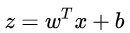) based on the classification, such as the classification task, ie What do we intuitively do? Most intuitively, you can put the output of a linear model on a function The simplest is the "unit-step function", as shown by the red line in the figure below.

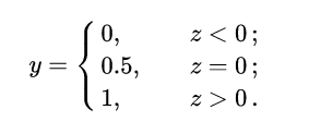
That is, As a split line, the decision of greater than z is category 0, and the decision of less than z is category 1.

However, such a piecewise function is not very good in mathematics, and it is neither continuous nor subtle. We know that the objective function is usually continuously differentiable when it comes to optimization tasks. How to improve it?

Here we use the logarithmic probability function (as shown by the black curve in the figure):

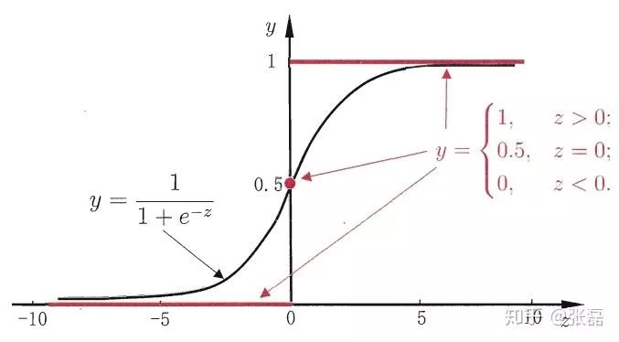
Unit step function and logarithmic probability function (from Zhou Zhihua's "machine learning")

It is a "Sigmoid" function, and the term "Sigmoid function" is a function that represents the form of an S-shaped function. The logarithmic probability function is one of the most important representations. This function has very good mathematical properties compared to the previous piecewise function. Its main advantages are as follows:

When using this function as a classification problem, not only the category can be predicted, but also an approximate probability prediction can be obtained. This is useful for many tasks that require the use of probabilistic aided decision making.

The logarithm probability function is an arbitrary order derivative function. It has very good mathematical properties. Many numerical optimization algorithms can be directly used to find the optimal solution.

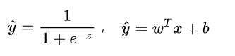
In general, the complete form of the model is as follows:

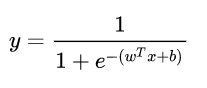
Actually, the LR model is fitting

1.2 Loss function

For any machine learning problem, it is necessary to specify the loss function first, and the LR model is no exception. When encountering the regression problem, we usually directly think of the following loss function form (mean square error loss MSE):

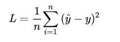
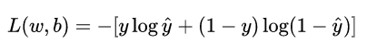
But what is the loss function in the two-class problem to be solved by the LR model? First give the form of this loss function, you can take a look at it and then explain it.

This loss function is usually called the log loss, where the logarithm base is the natural logarithm e, where the real value y is 0/1, and the presumed value Due to the logarithmic probability function, the output is a continuous probability value between 0 and 1. When you look closely, it is not difficult to find that when the real value y=0, the first item is 0. When the real value y=1, the second item is 0. Therefore, this loss function is always only one at a time in each calculation. If the item is working, can it not be converted to a piecewise function? The form of the piece is as follows:

It is not difficult to find that when the real value y is 1, the output value The closer to 1, the smaller L, the output value when the real value y is 0 The closer to 0, the smaller the L (you can draw your own hand The curve of the function). The piecewise function integration is followed by the logloss loss function listed above.

1.3 Optimization Solution

Now that we have determined the model's loss function, the next step is to continually optimize the model parameters based on this loss function to obtain the best model for fitting the data.

Revisit the loss function, which is essentially a function of L on the two parameters w and b of the linear equation part of the model:

among them,

The current learning task is transformed into a mathematically optimized form:

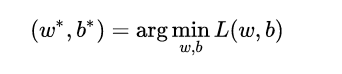
Since the loss function is continuously different, we can use the gradient descent method to perform the optimization solution. The update method for the core parameters is as follows:

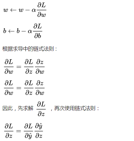
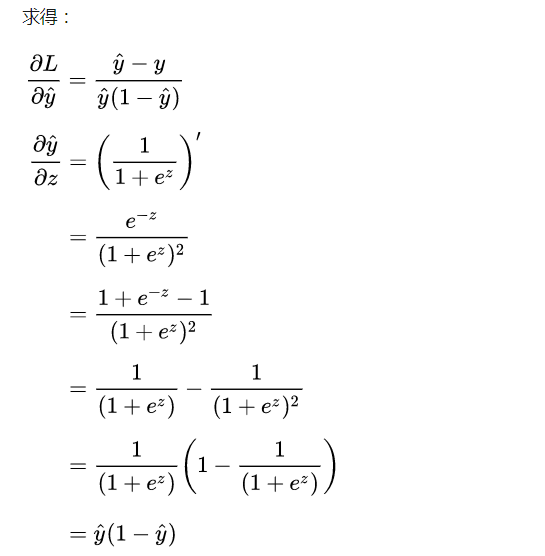
Here's an interesting thing to calculate:

Calculating a half-day turns out to be so simple, it is a guess The difference between the real value Y and this, in fact, is also due to the very mathematical nature of the logarithmic probability function itself.

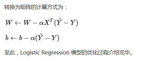
Make persistent efforts to obtain:

2 code to achieve

Below we begin to implement a simple LR model with python itself.

Complete code can refer to: [link]

First, build the logistic_regression.py file, build the class of the LR model, and internally implement its core optimization functions.

# -*- coding: utf-8 -*-import numpy as npclass LogisticRegression(object): def __init__(self, learning_rate=0.1, max_iter=100, seed=None): self.seed = seed self.lr = learning_rate self .max_iter = max_iter def fit(self, x, y): np.random.seed(self.seed) self.w = np.random.normal(loc=0.0, scale=1.0, size=x.shape[1] ) self.b = np.random.normal(loc=0.0, scale=1.0) self.x = x self.y = y for i in range(self.max_iter): self._update_step() # print('loss: {}'.format(self.loss())) # print('score: {}'.format(self.score())) # print('w: {}'.format(self.w)) # Print('b: {}'.format(self.b)) def _sigmoid(self, z): return 1.0 / (1.0 + np.exp(-z)) def _f(self, x, w, b): z = x.dot(w) + b return self._sigmoid(z) def predict_proba(self, x=None): if x is None: x = self.x y_pred = self._f(x, self.w, self .b) return y_pred def predict(self, x=None): if x is None: x = self.x y_pred_proba = self ._f(x, self.w, self.b) y_pred = np.array([0 if y_pred_proba[i] < 0.5 else 1 for i in range(len(y_pred_proba))]) return y_pred def score(self, y_true =None, y_pred=None): if y_true is None or y_pred is None: y_true = self.y y_pred = self.predict() acc = np.mean([1 if y_true[i] == y_pred[i] else 0 For i in range(len(y_true))]) return acc def loss(self, y_true=None, y_pred_proba=None): if y_true is None or y_pred_proba is None: y_true = self.y y_pred_proba = self.predict_proba() return Np.mean(-1.0 * (y_true * np.log(y_pred_proba) + (1.0 - y_true) * np.log(1.0 - y_pred_proba))) def _calc_gradient(self): y_pred = self.predict() d_w = (y_pred - self.y).dot(self.x) / len(self.y) d_b = np.mean(y_pred - self.y) return d_w, d_b def _update_step(self): d_w, d_b = self._calc_gradient() Self.w = self.w - self.lr * d_w self.b = self.b - self.lr * d_b return self.w, self.b

Then, here we created a file that was used alone to create simulation data and internally implemented training/test data partitioning.

# -*- coding: utf-8 -*-import numpy as npdef generate_data(seed): np.random.seed(seed) data_size_1 = 300 x1_1 = np.random.normal(loc=5.0, scale=1.0, size= Data_size_1) x2_1 = np.random.normal(loc=4.0, scale=1.0, size=data_size_1) y_1 = [0 for _ in range(data_size_1)] data_size_2 = 400 x1_2 = np.random.normal(loc=10.0, scale =2.0, size=data_size_2) x2_2 = np.random.normal(loc=8.0, scale=2.0, size=data_size_2) y_2 = [1 for _ in range(data_size_2)] x1 = np.concatenate((x1_1, x1_2) , axis=0) x2 = np.concatenate((x2_1, x2_2), axis=0) x = np.hstack((x1.reshape(-1,1), x2.reshape(-1,1))) y = np.concatenate((y_1, y_2), axis=0) data_size_all = data_size_1+data_size_2 shuffled_index = np.random.permutation(data_size_all) x = x[shuffled_index] y = y[shuffled_index] return x, ydef train_test_split(x, y): split_index = int(len(y)*0.7) x_train = x[:split_index] y_train = y[:split_index] x_test = x[split_index:] y_test = y[split_index:] return x_train, y_tr Ain, x_test, y_test

Finally, create the train.py file, call the LR class model you wrote earlier to implement the classification task, and view the accuracy of the classification.

# -*- coding: utf-8 -*-import numpy as npimport matplotlib.pyplot as pltimport data_helperfrom logistic_regression import *# data generationx, y = data_helper.generate_data(seed=272)x_train, y_train, x_test, y_test = data_helper.train_test_split (x, y)# visualize data# plt.scatter(x_train[:,0], x_train[:,1], c=y_train, marker='.')# plt.show()# plt.scatter(x_test[ :,0], x_test[:,1], c=y_test, marker='.')# plt.show()# data normalizationx_train = (x_train - np.min(x_train, axis=0)) / (np. Max(x_train, axis=0) - np.min(x_train, axis=0))x_test = (x_test - np.min(x_test, axis=0)) / (np.max(x_test, axis=0) - np .min(x_test, axis=0))# Logistic regression classifierclf = LogisticRegression(learning_rate=0.1, max_iter=500, seed=272)clf.fit(x_train, y_train)# plot the resultsplit_boundary_func = lambda x: (-clf.b - clf.w[0] * x) / clf.w[1]xx = np.arange(0.1, 0.6, 0.1)plt.scatter(x_train[:,0], x_train[:,1], c=y_train , marker='.') plt.plot(xx, split_boundary_func(xx), c='red')plt.show()# loss on test se Ty_test_pred = clf.predict(x_test)y_test_pred_proba = clf.predict_proba(x_test)print(clf.score(y_test, y_test_pred))print(clf.loss(y_test, y_test_pred_proba))# print(y_test_pred_proba)

The output result chart is as follows:

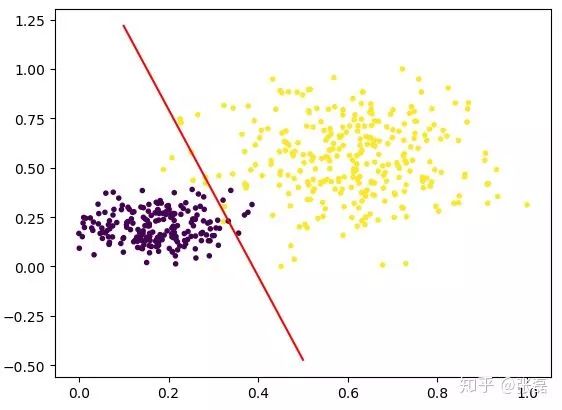
Output classification result graph

The red line is the linear equation in the LR model, so essentially what LR is doing is to continuously fit this red segmentation boundary so that the correctness of the classification on both sides of the boundary is as high as possible. Therefore, LR is actually a linear classifier. When the distribution of input data is nonlinear and complicated, we often need to adopt more complex models or continue to make a fuss about feature engineering.

Dell Adapter

Laptop power adapter charger for Dell:

Laptop Model	Adapter Output
Latitude E5400 E5410 E5500 E5510	19.5v 4.62a, 7450
Studio XPS 16 (1645)1640 1645 1647	19.5v 4.62a, 7450
Studio XPS M1645 M1647	19.5v 4.62a, 7450
XPS 14 15 17 L501x L502x L702x L702x	19.5v 4.62a, 7450
Inspiron 1464 1564 1764	19.5v 4.62a, 7450
Inspiron 1525 1440 1526	19.5v 3.34a, 7450
Precision M4600 M6600	19.5v 6.7a, 7450
Inspiron N5050 N4010 N5110	19.5v 3.34a, 7450
Inspiron 14Z-N411Z 13Z N311Z	19.5v 4.62a, 7450
Inspiron 1545	19.5v 3.34a, 7450
Latitude E5420 E5530 E5430 E6420	19.5v 4.62a, 7450
Inspiron 1440 1525 1526 1545 1750	19.5v 3.34a, Octagon tip
Inspiron 1300 B120 B130	19v 3.16a/3.42, 5525
Inspiron 1525 1526 1545	19.5v 3.34a, 7450
Studio 1440 1440n 1440z 14z 14zn	19.5v 3.34a, 7450
Latitude E4300 E4310	19.5v 4.62a, 7450
Inspiron 13Z 13ZD 13ZR M301 M301z M301ZD M301ZR N301	19.5v 3.34a, 7450
Inspiron N301Z N301ZD N301ZR	19.5v 3.34a, 7450
Studio 1535 1536 1555 1557 1558	19.5v 4.62a, 7450
Latitude E5420 E5520 E6430 E6530 E6420 E6520	19.5v 4.62a, 7450
Inspiron Mini 10 10v 1010 1010n 1010v 1011 1011n 1011v	19v 1.58a, 5517
Inspiron 14V 14VR M4010 N4020 N4030	19.5v 4.62a, 7450
Inspiron N4110 N5110 N7110 M5010	19.5v 3.34a, 7450
630M 640M E1405	19.5v 4.62a, 7450
Inspiron 15-3521 17-3721	19.5v 3.34a, 7450
Latitude 120L	19.5v 3.34a, 7450
Vostro 1710 1710n 1720 1720n	19.5v 4.62a, 7450
Vostro 1500 1700 Inspiron 1520 1521 1720	19.5v 4.62a, 7450
Vostro 1400 1420 PP26L	19.5v 3.34a, 7450
Latitude D410	19.5v 3.34a, 7450
Inspiron 1120, 1121, M101	19.5v 3.34a, 7450
Inspiron Mini 1012 1018	19v 1.58a, 5517

Our service:

Stable output and high charging efficiency.

Elegant outlook design as original one, touch smoothly and comfortable.

Original charger is good, but as a replacement, our product has more reasonable price when your original charger is broken.

And, the market of the replacement adapters becomes bigger and bigger. People would rather buy a copy one then the original because of the price.

But at the same time, people worry about that they will buy something defective. So the problem comes, how to buy a good quality one with a good price?

As a professional power adapter manufacturer, we have excellent R&D team, skilled staffs and responsible after-sale service. All your benefits can be under protected after you buy products for our company.

Our certificates :ISO9001:2008 & ISO14001:2004 , CCC , CE , FCC , ROHS.

All our products has 1 year warranty. In other words, if you get the dad products which are not damaged physically from us in one year, we will replace you the new one or the whole bulk order.

Mini Charger For Dell,Big Connector Adapter,45W Power Adapter,Dell Computer Adapter

Shenzhen Waweis Technology Co., Ltd. , https://www.huaweishiadapter.com