How can we efficiently train deep learning models?
In recent years, deep learning has achieved amazing results in NLP, image recognition, speech recognition, and machine translation. However, the application scope of deep learning is increasingly limited by the amount of data and the scale of the model. How can we efficiently train deep learning models? Based on a complete understanding of machine learning, Chen Wei, a researcher in charge of the machine learning group of Microsoft Research Asia, and her team closely combined distributed technology and deep learning to explore a new truly integrated "distributed deep learning" algorithm .
With the emergence of big data and efficient computing resources, deep learning has made major breakthroughs in many areas of artificial intelligence. However, in the face of increasingly complex tasks, the scale of data and deep learning models has become increasingly large. For example, the amount of labeled image data used to train image classifiers amounts to millions or even tens of millions. The emergence of large-scale training data provides a material basis for training large models. Therefore, many large-scale machine learning models have emerged in recent years, such as the LightLDA topic model developed by Microsoft Research Asia in 2015 with more than 20 billion parameters. . However, when the training data vocabulary grows to tens of millions, if no pruning is done, the deep learning model may have tens of billions, or even hundreds of billions of parameters.
In order to improve the training efficiency of deep learning models and reduce training time, we generally use distributed technology to perform training tasks-using multiple working nodes at the same time to train a neural network model with excellent performance in a distributed and efficient manner. Distributed technology is an accelerator of deep learning technology, which can significantly improve the training efficiency of deep learning and further increase its application range.
The goal of deep learning is to dig out patterns from data to help us make predictions. The general framework of deep learning algorithms is to use optimization algorithms to iteratively minimize the empirical risk on training data. Due to the statistical properties of data, the convergence properties of optimization, and the generalization properties of learning, the flexibility of multi-machine execution is higher. Compared with other computing tasks, deep learning algorithms do not actually need to be executed in parallel. The computing node strictly executes the single-machine version algorithm through communication. Therefore, when “distributed†encounters “deep learningâ€, it should not be limited to the technology of multi-machine implementation of serial algorithms and the underlying implementation. We should also integrate distributed and deep learning based on a complete understanding of machine learning. Learning is closely integrated, combined with the characteristics of deep learning, to design a new and truly integrated "distributed deep learning" algorithm.
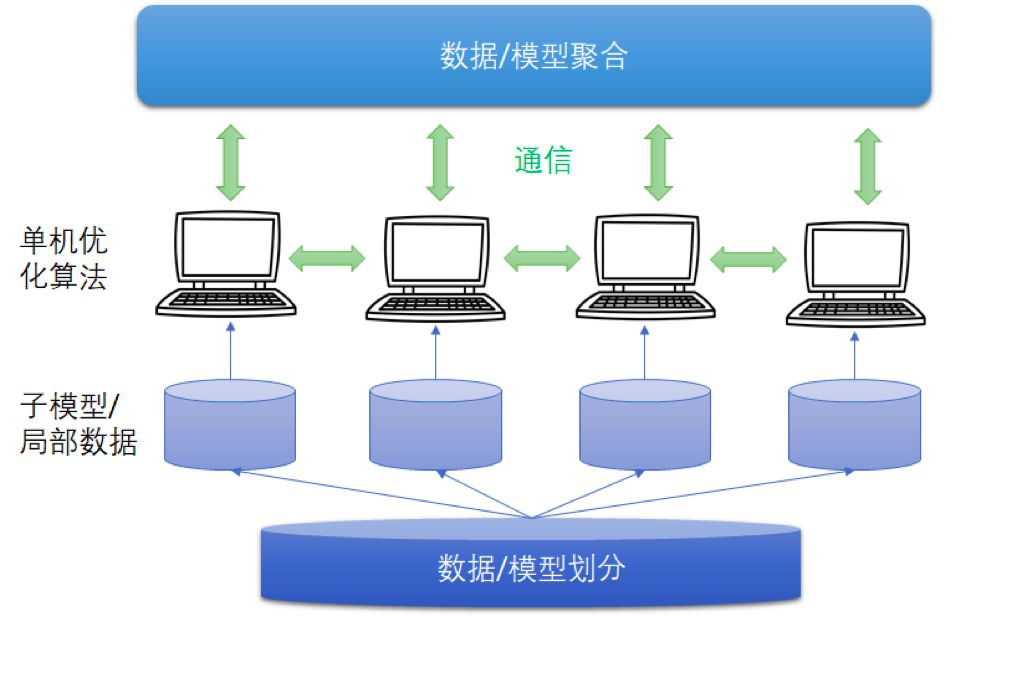
Figure 1 Distributed deep learning framework
The distributed deep learning framework includes modules such as data/model segmentation, local single-machine optimization algorithm training, communication mechanism, and data/model aggregation. Existing algorithms generally use data distribution methods of random scrambling and segmentation, local training algorithms of random optimization algorithms (such as stochastic gradient methods), synchronous or asynchronous communication mechanisms, and model aggregation methods of parameter averaging.
Combining the characteristics of deep learning algorithms, the machine learning team of Microsoft Asia Research Institute redesigned/understood these modules. We have mainly done three aspects of work in the field of distributed deep learning: the first work is aimed at gradient delay in asynchronous mechanisms Question, we designed an "asynchronous algorithm with delay compensation" for deep learning; in the second work, noting the non-convex nature of neural networks, we proposed an integrated aggregation method that is more effective than parameter averaging, and designed an "integrated -Compression" Parallel Deep Learning Algorithm; In the third work, we first analyzed the convergence rate of distributed deep learning algorithms under random scrambling and segmentation, and provided theoretical guidance for algorithm design.
DC-ASGD algorithm: Compensate the delay of gradient in asynchronous communication
Stochastic Gradient Descent (SGD) is currently one of the most popular deep learning optimization algorithms. The update formula is:
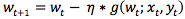
Formula 1
Among them, wt is the current model, (xt, yt) is randomly selected data, g(wt; xt, yt) is the gradient of the empirical loss function corresponding to (xt, yt) with respect to the current model wt, and η is the step size/ Learning rate.
Assuming that there are multiple working nodes in the system that use the stochastic gradient method to optimize the neural network model in parallel, synchronization and asynchronous are two commonly used communication synchronization mechanisms.
Synchronous SGD (Synchronous SGD), in each iteration of optimization, waits for all computing nodes to complete the gradient calculation, and then aggregates and averages the random gradients calculated on each working node, and updates the model according to Formula 1. After that, the working node receives the updated model and enters the next iteration. Since Sync SGD waits for all computing nodes to complete the gradient calculation, it is like a barrel effect. The calculation speed of Sync SGD will be dragged down by the work node with the lowest computational efficiency.
Asynchronous SGD (Asynchronous SGD) in each iteration, each working node directly updates the model after calculating the random gradient, no longer waiting for all computing nodes to complete the gradient calculation. Therefore, the asynchronous stochastic gradient descent method has a faster iteration speed and is also widely used in the training of deep neural networks. However, Async SGD is fast, but the gradient used to update the model is delayed, which will affect the accuracy of the algorithm. What is the "delay gradient"? Let's look at the picture below.
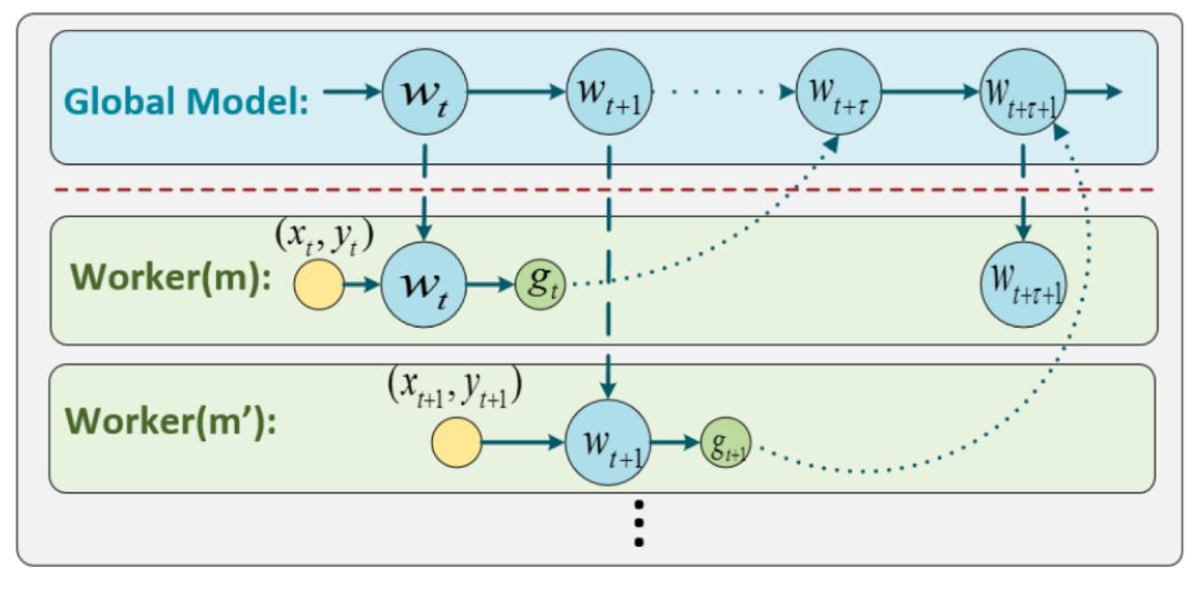
Figure 2 Asynchronous stochastic gradient descent method
During the operation of Async SGD, a worker node Worker(m) obtains the latest model parameter wt and data (xt, yt) at the beginning of the tth iteration, calculates the corresponding random gradient gt, and returns it to Update to the global model w. Since it takes a certain amount of time to calculate the gradient, when this working node returns the stochastic gradient gt, the model wt has been updated by other working nodes for Ï„ rounds and becomes wt+Ï„. In other words, the update formula of Async SGD is:

Formula 2
Compared with formula 1, the stochastic gradient used when updating the model wt+Ï„ in formula 2 is g(wt; xt, yt), which is compared with the stochastic gradient g(wt+Ï„; xt+Ï„, yt) that should be used in SGD +Ï„) produces a delay of Ï„ steps. Therefore, we call the stochastic gradient in Async SGD the "delay gradient".
The biggest problem caused by the delay gradient is that the gradient used to update the model each time is not the correct gradient (please note that g(wt; xt, yt) ≠g(wt+τ; xt+τ, yt+τ) ), so Async SGD will damage the accuracy of the model, and this phenomenon will become more and more serious as the number of machines increases. As shown in the figure below, as the number of computing nodes increases, the accuracy of Async SGD gradually deteriorates.

Figure 3 Performance of asynchronous stochastic gradient descent method
So, how can the asynchronous stochastic gradient descent method achieve higher accuracy while maintaining the training speed? We designed a DC-ASGD (Delay-compensated Async SGD) algorithm that can compensate for gradient delay.
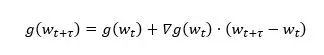
In order to study the relationship between the correct gradient g(wt+Ï„) and the delay gradient g(wt), we perform Taylor expansion of g(wt+Ï„) at wt:

Among them, ∇g(wt) is the gradient of the gradient, which is the Hessian matrix of the loss function, and H(g(wt)) is the Hessian matrix of the gradient. Obviously, the delay gradient is actually a zero-order approximation of the true gradient, and other items cause delay. Therefore, a natural idea is that if we calculate all the high-order terms, we can correct the delay gradient to an accurate gradient. However, since the remainder has infinite terms, it cannot be accurately calculated. Therefore, we choose to use the first-order term in the above formula for delay compensation:
As we all know, there are millions or more of parameters in modern deep neural network models. It is almost impossible to calculate and store the Hessian matrix ∇g(wt). Therefore, finding a good approximation of the Hessian matrix is ​​the key to whether the gradient delay can be compensated. According to the definition of Fisher information matrix, the outer product matrix of the gradient
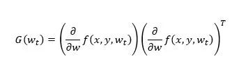
It is an asymptotically unbiased estimate of the Hessian matrix, so we choose G(wt) to approximate the Hessian matrix. According to previous studies, if the diagonal elements of the Hessian matrix are used to approximate the Hessian matrix in the neural network model, colleagues who significantly reduce the complexity of operation and storage can also maintain the accuracy of the algorithm, so we use diag(G(wt)) As an approximation of the Hessian matrix. In order to further reduce the approximate variance, we use a parameter λ between (0,1] to adjust the deviation and variance. In summary, we design the following asynchronous stochastic gradient descent method (DC-ASGD) with delay compensation,
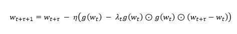
Among them, the compensation term for the delay gradient g(wt) contains only one step information, which hardly increases the calculation and storage costs.
We evaluated the DC-ASGD algorithm on the CIFAR10 data set and ImageNet data set. The experimental results are shown in the following two figures.
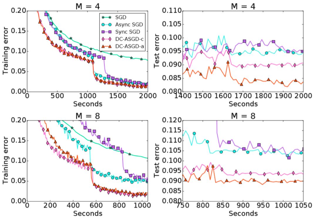
Figure 4 Training/test error of DC-ASGD_CIFAR-10
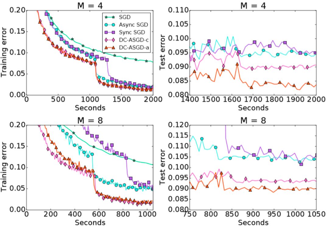
Figure 5 Training/test error of DC-ASGD_ImageNet
It can be observed that compared with the Async SGD algorithm, the DC-ASGD algorithm has a significant improvement in the accuracy of the model obtained in the same time, and it is also higher than the Sync SGD, which can basically achieve the same model accuracy as the SGD.
Ensemble-Compression algorithm: Improved aggregation method for non-convex models
Parameter average is a very common model aggregation method in existing distributed deep learning algorithms. If the loss function is convex with respect to the model parameters, the following inequality holds:
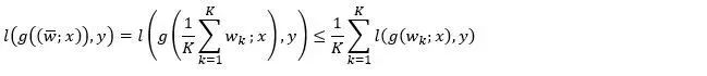
Among them, K is the number of computing nodes, wk is the local model, 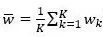 Is the model after parameter averaging, (x, y) is any sample data. The left end of the inequality is the loss function corresponding to the average model, and the right end is the average value of the loss function value of each local model. It can be seen that the average parameters in the convex problem can maintain the performance of the model.
However, for non-convex neural network models, the above inequality will no longer hold, so the performance of the average model is no longer guaranteed. This has also been verified experimentally: as shown in Figure 6, for different interaction frequencies (especially lower-frequency interactions), the average parameter usually greatly reduces the training accuracy, making the training process extremely unstable.
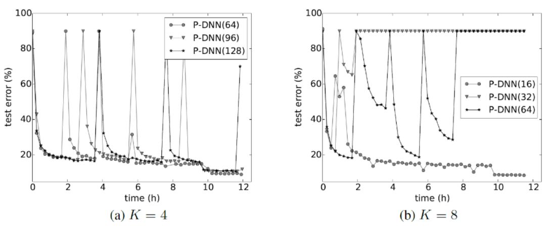
Figure 6 Distributed algorithm training curve based on parameter average (DNN model)
To solve this problem, we propose to replace model averaging with model integration as a model aggregation method in distributed deep learning. Although the loss function of the neural network is non-convex with respect to the model parameters, the output of the model is generally convex (such as the cross-entropy loss commonly used in deep learning). At this time, the following inequality can be obtained by using convexity:
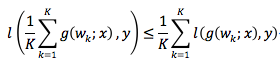
Among them, the left side of the inequality is the value of the loss function of the ensemble model. It can be seen that for non-convex models, the integrated model can maintain performance.
However, after each integration, the scale of the neural network model will double, and the problem of model scale explosion occurs. So, is there a way to use the advantages of model integration and avoid increasing the model? We propose a model aggregation method based on both model integration and model compression, namely the ensemble-compression method. After each integration, we compress the integrated model once.
The algorithm is specifically divided into three steps:
Each computing node trains a local model according to local optimization algorithm training and local data;
The local models communicate with each other between computing nodes to obtain the integrated model, and (part of) the local data are marked with the output value of the integrated model to them;
Using model compression technology (such as knowledge distillation), combined with the relabeling information of the data, model compression is performed on each working node separately, and a new model with the same size as the local model is obtained as the final aggregation model. In order to further save the amount of calculation, the process of distillation can be combined with the process of local model training.
This integration-compression aggregation method can not only achieve performance improvements through integration, but also maintain the scale of the global model during the iterative process of learning. The experimental results on CIFA-10 and ImageNet also verify the effectiveness of the integration-compression aggregation method (see Figure 7 and Figure 8). When the frequency of communication between working nodes is low, the parameter averaging method performs poorly, but the model integration-compression method can still achieve ideal results. This is because ensemble learning is more effective when the sub-models have diversity, and lower communication frequency will cause each local model to be more dispersed and stronger; at the same time, lower communication frequency means lower communication cost. Therefore, the model integration-compression method is more suitable for scenarios where the network environment is relatively poor.
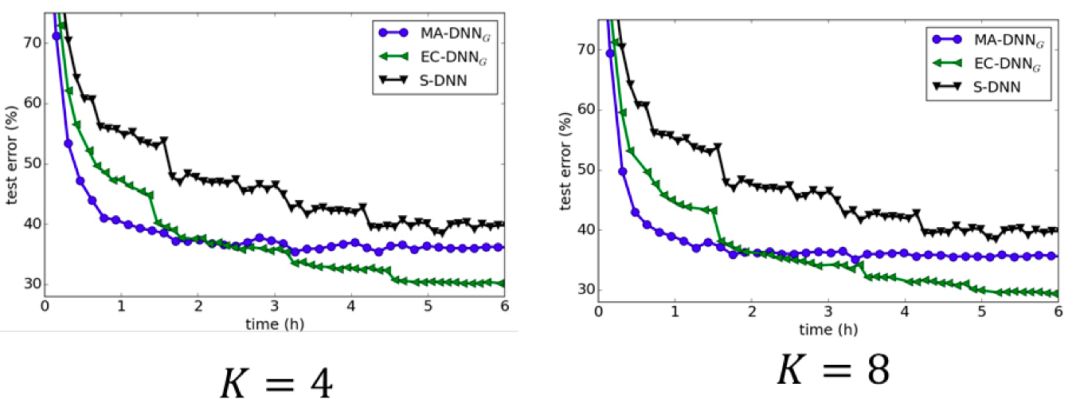
Figure 7 Comparison of various distributed algorithms on the CIFAR data set
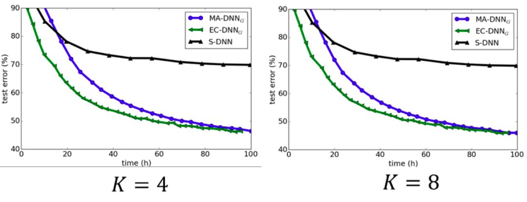
Figure 8 Comparison of various distributed algorithms on the ImageNet dataset
Distributed algorithm based on model integration is a relatively new research field, and there are still many unsolved problems. For example, when there are a large number of working nodes or the local model itself is large, the scale of the integrated model will become very large, which will bring about a large network overhead. In addition, when the integrated model is large, model compression will also become a large overhead. It is worth noting that at ICLR 2018, the Co-distillation method proposed by Hinton et al., although the motivation is different from this work, its algorithm is very similar to this work. How to understand these associations and solve these limitations will lead to new research, and interested readers can think about it.
Convergence analysis of algorithms under random rearrangement: improved distributed deep learning theory
Finally, a brief introduction to our recent work in improving distributed deep learning theory.
The commonly used data allocation strategy in distributed deep learning is to split equally after random rearrangement. Specifically, all training data is randomly shuffled to obtain a rearrangement of the data, and then the data set is divided into equal parts in order, and each copy is stored on the computing node. After the data has passed a round, if all the local data are collected and the above process is repeated, it is generally called "global rearrangement", if only the partial data is randomly rearranged, it is generally called "local rearrangement".
Most existing distributed deep learning theories assume that data is independent and identically distributed. However, the random rearrangement based on the Fisher-Yates algorithm is actually equivalent to sampling without replacement, and the training data is no longer independent and identically distributed. Therefore, the stochastic gradient calculated in each round is no longer an unbiased estimate of the exact gradient, so the theoretical analysis method of the previous distributed stochastic optimization algorithm is no longer applicable, and the existing convergence results may not still be valid.
We use Transductive Rademancher Complexity as a tool to give the upper bound of the deviation of the stochastic gradient relative to the exact gradient, and prove the convergence analysis of the distributed deep learning algorithm under random rearrangement.
Assuming that the objective function is smooth (not necessarily convex), there are K computing nodes in the system, the number of training rounds (epoch) is S, and there are n total training data, consider the distributed SGD algorithm.
(1) If the global random rearrangement data allocation strategy is adopted, the convergence rate of the algorithm is 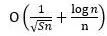 , Where the additional error caused by the non-iid nature is
  . Therefore, when the number of rounds of data is much smaller than the number of training samples (S ≪n), the impact of additional errors can be ignored. Considering that in existing distributed deep learning tasks, S ≪ n is easily satisfied, so global random rearrangement will not affect the convergence rate of distributed algorithms.
(2) If the local rearrangement strategy data distribution strategy is adopted, the convergence rate of the algorithm is 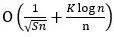 , Where the non-iid nature brings greater additional error
  . The reason is that because the random rearrangement is performed locally, and the data between different computing nodes is not interacted, the difference in the data is greater, and the deviation of the random gradient is also greater. When the number of rounds of data is S≪n/K2, the influence of additional errors can be ignored. In other words, when using the local rearrangement data distribution strategy, the number of rounds of data in the algorithm is affected by the number of computing nodes. If the number of computing nodes is relatively large, the number of passes cannot be too large.
At present, the field of distributed deep learning is developing very rapidly, and the above work is just some preliminary explorations done by our research group. I hope this article will enable more researchers to understand that "distributed" needs to be deeply integrated with "deep learning", and everyone will work together to promote the new development of distributed deep learning!
Insulated Power Cable,Bimetallic Crimp Lugs Cable,Pvc Copper Cable,Cable With Copper Tube Terminal
Taixing Longyi Terminals Co.,Ltd. , https://www.lycopperterminals.com