Want to understand recursive neural networks? Here is an introductory tutorial

Recursive neural network tutorial

introduction

Recurrent neural networks are artificial neural networks that can be used to identify patterns of sequences such as text, genomes, handwriting, speech, etc., and can also be used to identify numerical time series data generated by sensors, stock markets, and government agencies. The recursive network can be said to be the most powerful neural network. It can even decompose an image into a series of image blocks and process it as a sequence. Since the recursive network has a specific memory model, and memory is also one of the basic capabilities of human beings, the following will often compare the recursive network with the memory activities of the human brain.

Feedforward Network Review

To understand recursive networks, you first need to understand the basics of feedforward networks . The names of both networks come from the way they pass information through a series of network node mathematical operations. Feedforward networks deliver information straight ahead (never returning a node that has already passed), while recursive networks relay information.

In the feedforward network, the sample is converted into an output after entering the network; when supervised learning is performed, the output is a label. That is, the feedforward network maps the raw data to categories and identifies the pattern of the signal, such as whether a single input image should be labeled "cat" or "elephant."

We use a labeled image to shape a feedforward network until the network minimizes errors in guessing the image class. After the parameters, ie the weights, are shaped, the network can classify data that have never been seen before. The fixed feed-forward network can accept any random picture combination, and the first picture input does not affect the network's classification of the second picture. Seeing a picture of a cat does not cause the network to expect that the next picture is an elephant.

This is because the network does not have the concept of a time sequence, and the only input it considers is the currently accepted sample. Feed-forward networks seem to suffer from short-term amnesia; they only have memories that were previously stereotyped.

Recursive network

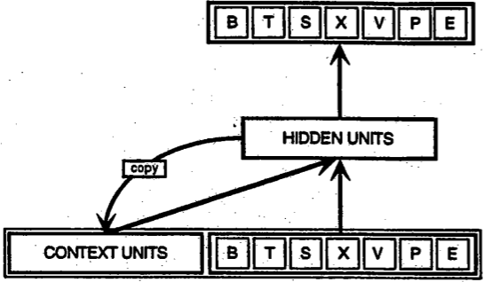
Recursive networks are different from feedforward networks in that their inputs include not only the input samples currently seen, but also the information the network has sensed at the previous moment. The following is a schematic diagram of [an early recursive network proposed by Elman] (https://web.stanford.edu/group/pdplab/pdphandbook/handbookch8.html). The bottom line BTSXPE in the figure represents the current input sample, and CONTEXT UNIT represents the output of the previous moment.

The decision of the recursive network at the t-1st time step will influence its decision at the tth subsequent time step. So the recursive network has two inputs from the present and the short time ago, the combination of the two determines how the network reacts to new data, which is quite similar to the situation in human daily life.

The difference between a recursive network and a feed-forward network lies in the feedback loop that continuously uses its own output as input. It is often said that recursive networks have memories. 2 The purpose of adding memory to a neural network is that the sequence itself carries information, and recursive networks can use this information to accomplish tasks that the feedforward network cannot accomplish.

These order information is stored in the hidden state of the recursive network, and is continuously transmitted to the front layer, which spans many time steps and affects the processing of each new sample.

Human memory will continue to make invisible cycles in the body, affecting our behavior without showing a complete appearance, and information will also circulate in the hidden state of the recursive network. There are many descriptions of the memory feedback loop in English. For example, we would say that "a person is entangled by what he used to do in the past." This is actually talking about the impact of past output on the current situation. The French called it "Le Passé qui ne passe pas", which means "The past has never passed."

Let us use mathematical language to describe the process of transferring memory forward:

The hidden state of the tth time step is h_t. It is a function of the input x_t of the same time step, modified by a weight matrix W (as we use in the feedforward network), plus the hidden state h_t-1 of the previous time step multiplied by its own hidden state - The U of the hidden state matrix (or the transition matrix, approximated by the Markov chain). The weight matrix is ​​a filter that determines how much importance is given to the current input and past hidden states. The error they produce will be returned by back-propagation and used to adjust the weight until the error can no longer be reduced.

The sum of the weighted input and the hidden state is squeezed with a function ?? - either a logical sigmoid function or a hyperbolic tangent function, depending on the situation - this is to compress a very large or small value to one Standard tools in logical space are also used to generate gradients that can be accepted by back propagation.

Since this feedback loop occurs at each time step in the series, each hidden state not only tracks the previous hidden state, but also includes all states prior to h_t-1 within the memory capability range.

If you enter a series of letters, the recursive network must determine the perception of the second character based on the first character. For example, if the first letter is q, the network may infer that the next letter is u, and the first If the letter is t, then the network may infer that the next letter is h.

Since the recursive network has a time dimension, it may be most clearly illustrated by an animation (the first occurrence of a vertical line of nodes may be regarded as a feed-forward network and become a recursive network as time progresses).

In the above figure, each x is an input sample, w is the weight used to filter the input, a is the activation state of the hidden layer (the sum of the input after the weight is added and the previous hidden state), and b is The output of the hidden layer after conversion, or "squeezing," uses linear correction or sigmoid units.

Backward propagation (BPTT)

As mentioned earlier, the purpose of recursive networks is to accurately classify the sequence input. We rely on error back propagation and gradient descent to achieve this goal.

The backward propagation of the feedforward network begins with the final error, and moves backward through each hidden layer's output, weight, and input, and assigns a certain percentage of error to each weight, by calculating the partial derivative of the weight and error- E/∂w, the ratio of the rate of change of the two. Subsequently, the gradient descent learning algorithm uses these partial derivatives to adjust the weights up and down to reduce errors.

Recursive networks use an extension of backpropagation, called backward propagation along time , or BPTT. Here, the time is actually expressed as a series of well-defined ordered calculations, connecting time steps one after the other, and these calculations are the entire contents of the back-propagation.

Whether recursive or not, neural networks are actually just nested composite functions of the form f(g(h(x))). Increasing the time element merely extends the series of functions. We use the chain rule to calculate the derivatives of these functions.

Truncated BPTT

Truncated BPTT is an approximation of a complete BPTT, and it is also a preferred choice when dealing with longer sequences. As the number of time steps is large, the forward/reverse calculation amount of each parameter update of the complete BPTT becomes very high. The disadvantage of this method is that due to the truncation operation, the distance of the gradient backward movement is limited, so the network can learn the dependency length shorter than the complete BPTT.

Gradient disappears (with expansion)

Like most neural networks, recursive networks are not new. In the early 1990s, the disappearance of gradients became a major obstacle to the performance of recursive networks.

Just as the straight line represents how x changes with y, the gradient represents the change in the weight of ownership as the error changes. If the gradient is unknown, you cannot adjust the weight in the direction of reducing the error and the network will stop learning.

Recursive networks have encountered major obstacles in finding the link between the final output and many events before the time step, because it is difficult to determine how much importance should be given to remote input. (These inputs, like those grandparents who once had ..., tend to increase rapidly as they continue to trace back, leaving behind an impression that is often vague.)

One of the reasons is that the information flowing in neural networks goes through many levels of multiplication.

Everyone who has studied compound interest rates knows that any number that is multiplied by a number that is slightly larger than one will increase to an incomprehensible point. (This is precisely the network effect in economics and the inevitable social inequality. A simple mathematical truth. The reverse is also true: multiplying a number by a number less than one can have the opposite effect. If the gambler loses 97 cents for every dollar note, that moment will go bankrupt.

Since the layers and time steps of the deep neural network are related to each other through multiplication, the derivative may disappear or expand.

When the gradient swells, each weight appears to be a butterfly mentioned in a proverb. When all the butterflies flap their wings together, they will trigger a hurricane in a distant place. The gradient of these weights increases to saturation, ie their importance is set too high. However, the gradient expansion problem is relatively easy to solve because it can be cut or squeezed. The disappearance of the gradient may become too small, so that the computer can not handle, the network can not learn - this problem is more difficult to solve.

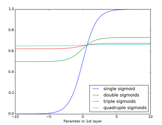
The result of applying the sigmoid function repeatedly is shown in the figure below. The data curve becomes more and more gentle until no inclination can be detected over a longer distance. The gradient disappears after passing through many layers.

Long Term Short Term Memory Unit (LSTM)

In the mid-1990s, the German scholars Sepp Hochreiter and Juergen Schmidhuber proposed a variant of the recursive network, with so-called long-short-term memory units, or LSTM, that can solve the problem of gradient disappearance.

LSTM preserves errors for reverse transfer along time and layers. LSTM keeps the error at a more constant level, allowing the recursive network to perform many time-steps of learning (over 1000 time steps), thus opening the way to establish long-distance causal links.

LSTM stores information in gated units outside the normal flow of recursive networks. These units can store, write or read information just like data in the computer's memory. The unit determines which information is stored by the switch of the door and when it is allowed to read, write or clear the information. However, unlike digital memories in computers, these gates are analog and contain element-by-element multiplication of sigmoid functions whose output ranges are all between 0 and 1. Compared to digital storage, analog values ​​have the advantage of being differentiable and are therefore suitable for back propagation.

These gates switch on the basis of the received signal, and similar to the nodes of the neural network, they use their own set of weights to filter the information and decide whether to allow the information to pass based on their strength and the content of the import. These weights, like the weights of modulation inputs and hidden states, are adjusted through the recursive network learning process. That is, the memory unit learns when the data is allowed to enter, leave, or be deleted by guessing, back propagation of the error, and an iterative process of adjusting the weight with gradient descent.

The figure below shows how the data flows in the memory unit and how the gates in the unit control the flow of data.

The content in the above picture is quite a lot. If readers just start learning LSTM, don't rush to read down - please take a moment to think about this picture. Just a few minutes, you will understand the secrets.

First, the bottom three arrows indicate that information flows from multiple points into the memory unit. The current input and past cell states are not only sent to the memory cell itself, but also to the three cells of the cell, and these gates will determine how to handle the input.

The black dots in the figure are gates that determine when to allow new inputs to enter, when to clear the current cell state, and/or when to have the cell state affect the network output of the current time step. S_c is the current state of the memory cell, and g_y_in is the current input. Remember, each door can be opened or closed, and the door will be re-switched at each time step. The memory unit can decide at each time step whether to forget its state, whether to allow writing, whether to allow reading, and the corresponding information flow is as shown in the figure.

The larger bold letters in the figure are the result of each operation.

Below is another diagram comparing simple recursive networks (left) with LSTM units (right). The blue line can be ignored; the legend helps to understand.

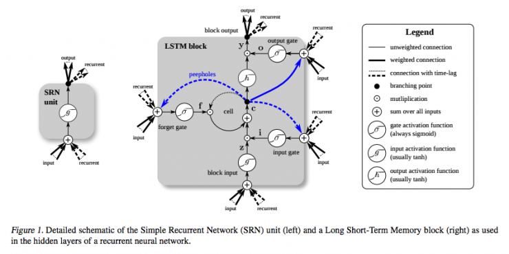
It should be noted that the LSTM's memory unit gives different roles for addition and multiplication in input conversion. The plus sign in the middle of the two figures is actually the secret of LSTM. Although seemingly simple, this basic change can help LSTM maintain a constant error when deep back propagation is necessary. The way LSTM determines the status of subsequent units is not to multiply the current state with the new input, but to add both, which is what LSTM is all about. (Of course, oblivion still uses multiplication.)

Different sets of weights filter input information and decide whether to input, output, or forget. The form of oblivion gate is a linear identity function, because if the gate is open, the current state of the memory cell will only be multiplied by 1 and propagated forward one time step.

In addition, when it comes to simple tips, setting the deviation of the forgotten gate of each LSTM unit to 1 has been proven to improve network performance. (But Sutskever suggests setting a bias of 5.)

You may ask, if the purpose of the LSTM is to link remote events with the final output, why do you need oblivion gates? Because sometimes forgetting is a good thing. To analyze a text corpus as an example, when you reach the end of the document, you may think that the next document is definitely not related to this document, so the memory unit should be zeroed before it starts absorbing the first element of the next document.

In the figure below you can see how the door works, where the horizontal lines represent the closed doors and the small hollow circles represent the open doors. Horizontal lines and circles below the hidden layer are oblivious gates.

It should be noted that the feedforward network can only map one input to one output, while the recursive network can map one input to multiple outputs (from one image to many words in the title) as shown in the figure above. Many-to-many (translation) or multiple-to-one (voice classification) mapping.

Covers multiple time scales and distance dependencies

You may also ask, the input gate prevents new data from entering the memory cell, and the output gate prevents the memory cell from affecting the RNN specific output. What is the exact value of these two gates? It can be considered that LSTM is equivalent to allowing a neural network to operate on different time scales simultaneously.

Take a person’s life as an example. Imagine how we can receive a different stream of data about this life in the form of a time series. In terms of geographical location, the location of each time step is important for the next time step, so the geographical time scale is always open to the latest information.

Assume that this person is a model citizen and will vote every few years. As far as the time scale of democratic life is concerned, we wish to pay special attention to what this person did before and after the election, and pay attention to what this person did before leaving a major issue and returning to daily life. We do not want our political analysis to be disturbed by the continuously updated geographical information.

If this person is still a model daughter, then we may be able to increase the time scale of family life, understand that the model she calls is once a week, and the number of calls will increase significantly during the annual festival. This has nothing to do with the cycle and geographical location of political activities.

The same is true for other data. Music has complex beats. The text contains topics that recur at different intervals. The stock market and the economy will experience short-term shocks in addition to long-term fluctuations. These events occur simultaneously on different time scales, and LSTM can cover all of these time scales.

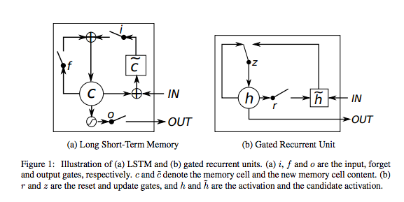
Gated recursion unit (GRU)

A gated recursive unit (GRU) is essentially an LSTM with no output gate, so it writes all the contents of the memory cell to the entire network at each time step.

LSTM hyperparameter debugging

The following are some things to note when manually optimizing RNN hyperparameters:

Careful overfitting has occurred, which is usually because the neural network is "dead" typing data. Overfitting means that the stereotyped data will perform well, but the network model is completely useless for predictions other than the sample.

Regularization is good: regularization methods include l1, l2, and discarding methods.

Keep a separate set of tests that the neural network does not finalize.

The larger the network, the stronger the function, but it is also easier to overfit. Don't try to learn a million parameters with 10,000 samples Parameter > Samples = Problem.

The data is basically always better, as it helps to prevent over-fitting.

Stereotypes should include multiple epochs (using the entire dataset to shape once).

After each epoch, evaluate the test set performance and determine when to stop (early stop).

The learning rate is the most important hyperparameter. Deeplearning4j-ui debugging; see this figure

In general, stacking layers are good.

For LSTM, use the softsign (rather than softmax) activation function instead of tanh (faster and less prone to saturation (approximately 0 gradient)).

Updater: RMSProp, AdaGrad, or momentum (Nesterovs) are usually better choices. AdaGrad can also attenuate learning rates and can sometimes help.

Finally, keep in mind data normalization, MSE loss function + identity activation function for regression, Xavier weight initialization

Note:

1) Although recursive networks may be far from universal artificial intelligence, we believe that intelligence is actually “stupid” than we think. In other words, with a simple feedback loop as a memory, we have one of the basic elements of consciousness - a necessary but insufficient condition. Other conditions not mentioned above may include additional variables that represent the network and its status, and a decision logic framework based on data interpretation. Ideally, the latter would be part of a larger problem-solving cycle, rewarding success, penalizing failure, and being very similar to reinforcement learning. Saying that DeepMind has created such a framework...

2) Neural networks with optimized parameters all have memories in a sense because these parameters are traces of historical data. But in feed-forward networks, this memory may be frozen in the past. In other words, when the network is finalized, the model it learns may be applied to more data and no longer adjust itself. In addition, this type of network is also unique in that it uses the same memory (or set of weights) for all input data. Recursive networks are also sometimes referred to as dynamic (meaning: "evolving") neural networks. The biggest difference between feedforward networks and feedforward networks is not the possession of memory, but the ability to assign specific weights to multiple events that occur in a sequence. Although these events do not necessarily need to be closely linked, the network will assume that they are all linked by the same timeline, no matter how far away. Feedforward networks do not make such assumptions. They see the world as a bunch of objects that do not have a chronological order. Comparing these two neural networks with two human knowledge may help to understand. When we were young, we learned to recognize colors, and then we recognized all colors wherever we were in our lives. This was true in all kinds of situations that were extremely different, and it was not influenced by time. We only need to learn color once. This kind of knowledge is like the memory of feed-forward networks: they rely on a kind of past information with no scope and no limit. They do not know or care what color was entered five minutes ago. The feed-forward network has short-term amnesia. On the other hand, when we were young, we would also learn how to interpret the flow of sound signals called languages. The meanings we extract from these sounds, such as “toe”, “roe” or “z”, are always highly dependent on The sound signal appears. Each step of the sequence is based on the previous step, and meaning is generated in their order. Indeed, the meaning of each syllable in a sentence is conveyed by many whole sentences, and the redundant signal in the sentence is protected against environmental noise. The memory of recursive networks is similar to this and they rely on a specific piece of past information. Both networks make different past information work in different ways.

Reproduced from DEEPLEARNING4J, Lei Feng network (search "Lei Feng network" public number concerned) compile